

The days of manually calculating formulas are long gone for accountants. Not only do accountants have calculators at their disposal, but they also have the bread and butter of the industry: Excel. Excel is an accountant’s best friend, helping sort data and solve complex formulas.
Whether you are new to the accounting industry or are looking to level up your Excel game, here are 10 Excel accounting formulas every accountant should know.
1: SUMIF
Formula: =SUMIF(range, criteria, sum range)
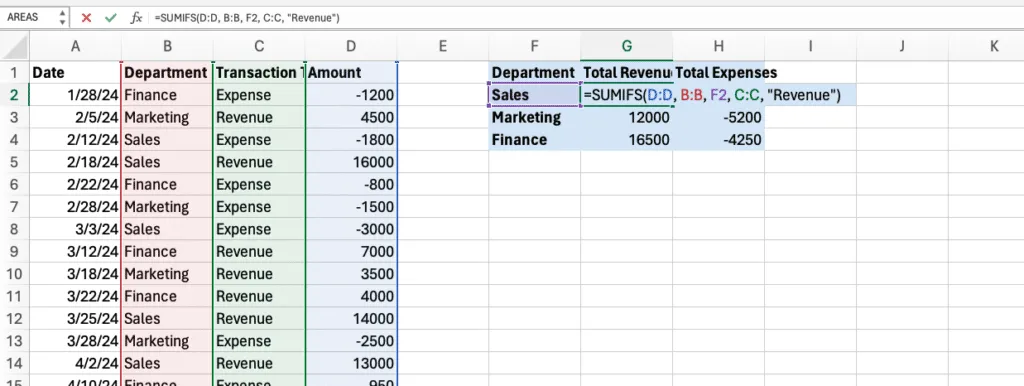
It’s not uncommon for accountants to receive data piled into one Excel spreadsheet. Instead of manually totaling line items, the SUMIF formula does this for you. All you need to do is identify the range of data you want to sum, the criteria, and select the sum range. This formula adds up values if they meet the criteria, which could be a specific number, value, or word. For example, if you are trying to see how much maintenance expenses are in the spreadsheet, SUMIF would pick out all of the dollar amounts that are coded to maintenance.
2: IF
Formula: =IF(logical test, value if true, value if false)
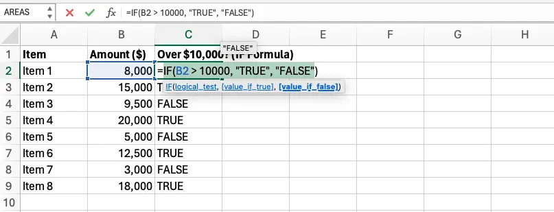
The IF function allows you to ask a question and receive a true or false answer. For example, you might go through a data set and ask the IF function to pick out values over $10,000. If the line item is over the amount, it will default to “True” in the box. On the flip side, if the value is under $10,000, the box will say “False.” By defaulting data to true or false, you can pick out which values you need to pay attention to. For example, if your materiality threshold is $15,000, you wouldn’t care about any line items that contain less than this amount.
3: ROUNDUP
Formula: =ROUNDUP(number, number digits)
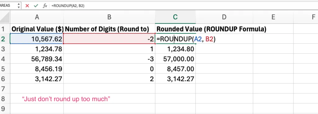
The ROUNDUP formula is important when you don’t care about decimal values. This formula gives you the ability to switch values to flat numbers. For example, $10,567.62 might be rounded up to $10,600. Rounding up to flat numbers makes the data easier to digest. In the number digits section, you will enter how many places you want the number to round up. For example, putting -2, would round our example number up to $10,600, while three spots would round it up to $11,000.
Note: this can also be achieved through formatting.
4: PMT
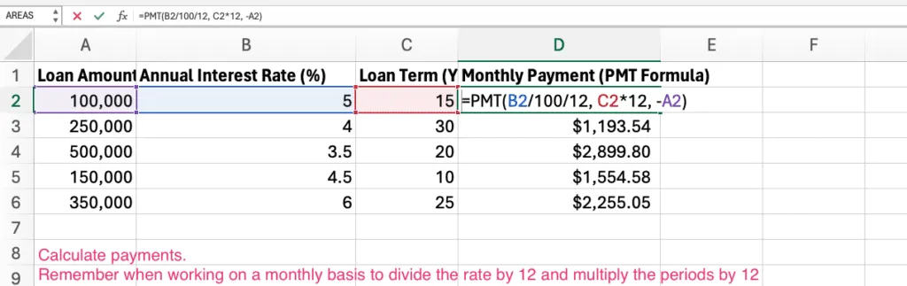
Formula: =PMT(rate, number of periods, present value)
The PMT function is commonly used for accountants who work with real estate financial models. This formula gives you the monthly payment based on defined criteria, including the rate, number of periods, and present value. Instead of using a separate mortgage calculator, accountants can use the PMT function to keep all data and formulas in one place.
* Remember when working on a monthly basis to divide the rate by 12 and multiply the periods by 12.
5: XNPV
Formula: =XNPV(discount rate, cash flows, dates)
The XNPV formula is one of the most useful formulas for accountants. It helps you determine the projected profitability of an investment. A high NPV indicates that the investment will generate a higher return than the required rate of return. For example, if you are considering purchasing a real estate investment, you could enter your tentative cash flow with the discount rate to determine a fair purchase price.
6: SLN
Formula: =SLN(cost, salvage value, life)
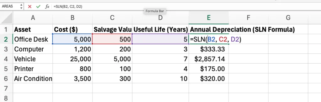
One of the main roles of an accountant is to handle fixed assets and depreciation. For book purposes, most assets will be depreciated using straight-line depreciation over the useful life. Excel can calculate the straight-line depreciation of an asset. You will need the asset’s cost, the price you expect to sell it for after the useful life, and the useful life. Remember, this formula may need to be pro-rated based on when the asset is placed in service, as the formula will calculate a full year of depreciation.
7: RATE
Formula: =RATE(number of payment periods, annual amount of payments, present value of loan, loan balance after last payment, type, guess)
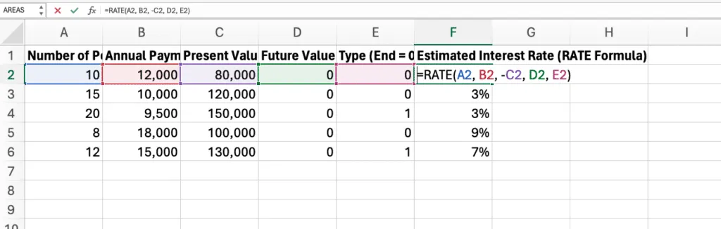
The RATE formula computes the loan interest rate, or the rate of return needed to reach a specific amount on an investment. For this formula to work, all value entries need to be numeric. For example, you must type 4, not four. Using this formula is common to see the average annual financing cost on multiple loans.
8: FV
Formula: =FV(rate, number of payment periods, payment, value of future payments, type)
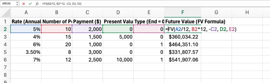
The FV formula is used by accountants to determine how much value an investment will have in the future. This formula is only effective if payments are consistent. For example, this formula would not generate accurate results for a rental property that increases rent each year. However, it would be beneficial to calculate the return on a CD or bond.
9: MIRR
Formula: =MIRR(cash flows, finance rate, reinvest rate)
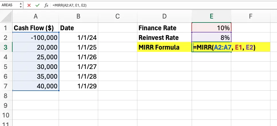
The MIRR formula calculates the modified internal rate of return on investments by including reinvested proceeds. This calculation is beneficial to understand the potential profitability of an investment or project. The finance rate and the reinvestment rate will be expressed as a decimal point. For example, an 8% return would be inputted as 0.08. Using MIRR allows accountants to easily calculate internal rates of returns on different projects to select the best fit.
10: VLOOKUP
Formula: =VLOOKUP(table value, table array, column index, range lookup)
The VLOOKUP function searches for a value in a table based on the value from a specific column. This formula is helpful for looking up a price based on the general ledger code or individual number or for moving information from one sheet to another. For example, an accountant might use this to total all values with the same general ledger code. A similar formula to VLOOKUP is XLOOKUP.
Summary
These 10 formulas are important to know as an accountant, whether you are working in public accounting or an industry sector. By integrating these items into your daily to-do’s, you can infuse efficiency and accuracy into your calculations. You don’t need to worry about triple-checking formulas or manual calculations. Instead, Excel computes most of the backend work on your behalf.